Introducing tidygraph
July 7, 2017
I’m very pleased to announce that my new package tidygraph is now
available on CRAN. As the name
suggests, tidygraph is an entry into the tidyverse that provides a tidy
framework for all things relational (networks/graphs, trees, etc.). tidygraph
is a relatively big package in terms of exported functions (280 exported
symbols) so all functions will not be covered in this release note. I will
however provide an overview of all the areas that tidygraphtouches upon so you
should have a pretty good grasp on what the package can do for you.
Tidy network data?
There’s a discrepancy between relational data and the tidy data idea, in that relational data cannot in any meaningful way be encoded as a single tidy data frame. On the other hand, both node and edge data by itself fits very well within the tidy concept as each node and edge is, in a sense, a single observation. Thus, a close approximation of tidyness for relational data is two tidy data frames, one describing the node data and one describing the edge data.
The tbl_graph object
Underneath the hood of tidygraph lies the well-oiled machinery of igraph,
ensuring efficient graph manipulation. Rather than keeping the node and edge
data in a list and creating igraph objects on the fly when needed, tidygraph
subclasses igraph with the tbl_graph class and simply exposes it in a tidy
manner. This ensures that all your beloved algorithms that expects igraph
objects still works with tbl_graph objects. Further, tidygraph is very
careful not to override any of igraphs exports so the two packages can coexist
quite happily.
To underline the tidyness of the tbl_graph class the print method shows the
object as two tibbles along with additional network information.
library(tidygraph)
create_ring(10)
#> # A tbl_graph: 10 nodes and 10 edges
#> #
#> # An undirected simple graph with 1 component
#> #
#> # Node Data: 10 x 0 (active)
#> #
#> # Edge Data: 10 x 2
#> from to
#> <int> <int>
#> 1 1 2
#> 2 2 3
#> 3 3 4
#> # ... with 7 more rowstbl_graph objects can be created directly using the tbl_graph() function
that takes a node data.frame and an edge data.frame. On top of that, tidygraph
also provides coercion from a huge amount of relational data structures. The
following list gives the packages/classes that can currently be converted to
tbl_graphs, using the as_tbl_graph function:
data.frame,list,matrixfrombaseigraphfromigraphnetworkfromnetworkdendrogramandhclustfromstatsNodefromdata.treephyloandevonetfromapegraphNEL,graphAM,graphBAMfromgraph(in Bioconductor)
For all of the coercions you can expect that data on the nodes and edges are
kept and available after conversion to tbl_graph:
iris_clust <- hclust(dist(iris[1:4]))
iris_tree <- as_tbl_graph(iris_clust)
iris_tree
#> # A tbl_graph: 299 nodes and 298 edges
#> #
#> # A rooted tree
#> #
#> # Node Data: 299 x 4 (active)
#> height leaf label members
#> <dbl> <lgl> <fctr> <int>
#> 1 0.0000000 TRUE 108 1
#> 2 0.0000000 TRUE 131 1
#> 3 0.2645751 FALSE 2
#> 4 0.0000000 TRUE 103 1
#> 5 0.0000000 TRUE 126 1
#> 6 0.0000000 TRUE 130 1
#> # ... with 293 more rows
#> #
#> # Edge Data: 298 x 2
#> from to
#> <int> <int>
#> 1 3 1
#> 2 3 2
#> 3 7 5
#> # ... with 295 more rowsLastly, tidygraph also wraps the multitude of graph constructors available in
igraph and exports them under the create_*() family of functions for
deterministic constructors (e.g. the call to create_ring(10) above) and the
play_*() family for constructors that incorporate sampling (e.g.
play_erdos_renyi() for creating graphs with a fixed edge probability). All of
these functions provide a consistent argument naming scheme to make them easier
to use and understand.
Meet a new verb…
There are many ways a multitable setup could fit into the tidyverse. There could
be an added qualifier to the verbs such as mutate_nodes() and filter_edges()
or each verb could take an additional argument specifying what is targeted e.g.
arrange(..., target = 'nodes'). Both of these approachable are viable but
would require a huge amount of typing as well as being taxing to support down
the line.
The approach used by tidygraph is to let the data object itself carry around
a pointer to the active data frame that should be the target of manipulation.
This pointer is changed using the activate() verb, which, on top of changing
which part of the data is being worked on, also changes the print output to show
the currently active data on top:
iris_tree %>% activate(edges)#> # A tbl_graph: 299 nodes and 298 edges
#> #
#> # A rooted tree
#> #
#> # Edge Data: 298 x 2 (active)
#> from to
#> <int> <int>
#> 1 3 1
#> 2 3 2
#> 3 7 5
#> 4 7 6
#> 5 8 4
#> 6 8 7
#> # ... with 292 more rows
#> #
#> # Node Data: 299 x 4
#> height leaf label members
#> <dbl> <lgl> <fctr> <int>
#> 1 0.0000000 TRUE 108 1
#> 2 0.0000000 TRUE 131 1
#> 3 0.2645751 FALSE 2
#> # ... with 296 more rowsAs can be seen, activate() takes a single argument specifying the part of the
data that should be targeted for subsequent operations as an unquoted symbol.
tidygraph continues the naming conventions from ggraph using nodes and
edges to denote the entities and their connections respectively, but
vertices and links are allowed synonyms inside activate().
The current active data can always be extracted as a tibble using as_tibble()
as_tibble(iris_tree)#> # A tibble: 299 x 4
#> height leaf label members
#> <dbl> <lgl> <fctr> <int>
#> 1 0.0000000 TRUE 108 1
#> 2 0.0000000 TRUE 131 1
#> 3 0.2645751 FALSE 2
#> 4 0.0000000 TRUE 103 1
#> 5 0.0000000 TRUE 126 1
#> 6 0.0000000 TRUE 130 1
#> 7 0.3464102 FALSE 2
#> 8 0.5196152 FALSE 3
#> 9 0.5567764 FALSE 5
#> 10 0.0000000 TRUE 119 1
#> # ... with 289 more rowsThe dplyr verbs
Using activate() it is possible to use the well known dplyr verbs as one
would expect without much hassle:
iris_tree <- iris_tree %>%
    activate(nodes) %>%
    mutate(Species = ifelse(leaf, as.character(iris$Species)[label], NA)) %>%
    activate(edges) %>%
    mutate(to_setose = .N()$Species[to] == 'setosa')
iris_tree
#> # A tbl_graph: 299 nodes and 298 edges
#> #
#> # A rooted tree
#> #
#> # Edge Data: 298 x 3 (active)
#> from to to_setose
#> <int> <int> <lgl>
#> 1 3 1 TRUE
#> 2 3 2 TRUE
#> 3 7 5 TRUE
#> 4 7 6 TRUE
#> 5 8 4 TRUE
#> 6 8 7 NA
#> # ... with 292 more rows
#> #
#> # Node Data: 299 x 5
#> height leaf label members Species
#> <dbl> <lgl> <fctr> <int> <chr>
#> 1 0.0000000 TRUE 108 1 setosa
#> 2 0.0000000 TRUE 131 1 setosa
#> 3 0.2645751 FALSE 2 <NA>
#> # ... with 296 more rowsIn the above the .N() function is used to gain access to the node data while
manipulating the edge data. Similarly .E() will give you the edge data and
.G() will give you the tbl_graph object itself.
Some verbs have effects outside of the currently active data.
filter()/slice() on node data will remove the edges terminating at the
removed nodes and arrange() on nodes will change the indexes of the to and
from column in the edge data.
While one might expect all of dplyrs verbs to be supported in that manner,
there is a clear limitation in the relational data structure that requires rows
to maintain their identity. Thus, summarise() and do() are not allowed as
there is no clear interpretation of how alterations on the node and edge data
with these verbs should be interpreted. If these operations are required I
suggest applying them to a tibble representation and then joining the result
back in.
Speaking of joining, all joins from dplyr are supported. Nodes and edges are
added and removed as required by the join. New edge data to be joined in must
have a to and from column referencing valid nodes in the existing graph.
library(dplyr)
iris_sum <- iris %>%
    group_by(Species) %>%
    summarise_all(mean) %>%
    ungroup()
iris_tree <- iris_tree %>%
    activate(nodes) %>%
    left_join(iris_sum)
iris_tree
#> # A tbl_graph: 299 nodes and 298 edges
#> #
#> # A rooted tree
#> #
#> # Node Data: 299 x 9 (active)
#> height leaf label members Species Sepal.Length Sepal.Width
#> <dbl> <lgl> <fctr> <int> <chr> <dbl> <dbl>
#> 1 0.0000000 TRUE 108 1 setosa 5.006 3.428
#> 2 0.0000000 TRUE 131 1 setosa 5.006 3.428
#> 3 0.2645751 FALSE 2 <NA> NA NA
#> 4 0.0000000 TRUE 103 1 setosa 5.006 3.428
#> 5 0.0000000 TRUE 126 1 setosa 5.006 3.428
#> 6 0.0000000 TRUE 130 1 setosa 5.006 3.428
#> # ... with 293 more rows, and 2 more variables: Petal.Length <dbl>,
#> # Petal.Width <dbl>
#> #
#> # Edge Data: 298 x 3
#> from to to_setose
#> <int> <int> <lgl>
#> 1 3 1 TRUE
#> 2 3 2 TRUE
#> 3 7 5 TRUE
#> # ... with 295 more rowsExpanding the vocabulary
On top of what has been showed so far, tidygraph provides an assortment of
graph specific verbs that can be used to power your analysis and manipulation.
Analogous to bind_rows(), tidygraph provides three functions to expand your
data: bind_nodes() and bind_edges() append nodes and edges to the graph
respectively. As with the join functions bind_edges() must contain valid
from and to columns. bind_graphs() allows you to combine multiple graphs
in the same graph structure resulting in each original graph to become a
component in the returned graph.
While bind_graphs() cannot be used to create edges between the merged graphs
graph_join() can do just that. It merges nodes using a full_join() semantic
and keeps the individual edges from both graphs:
library(ggraph)
gr1 <- create_notable('bull') %>%
    mutate(name = letters[1:5])
gr2 <- create_ring(5) %>%
    mutate(name = letters[4:8])

# Plot
gr1 %>% bind_graphs(gr2) %>%
    ggraph(layout = 'kk') +
    geom_edge_link() +
    geom_node_point(size = 8, colour = 'steelblue') +
    geom_node_text(aes(label = name), colour = 'white', vjust = 0.4) +
    ggtitle('Binding graphs') +
    theme_graph()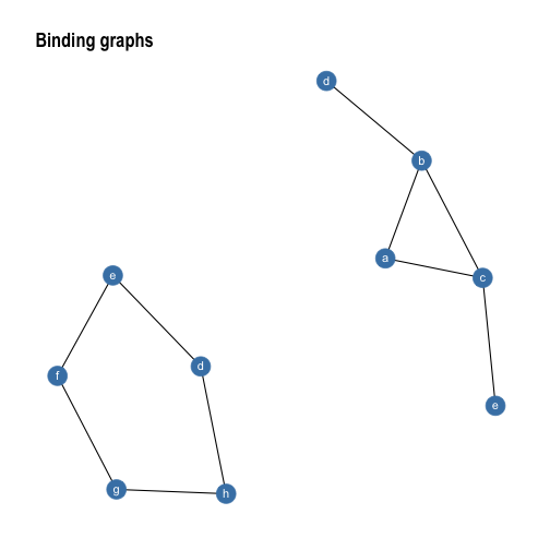
gr1 %>% graph_join(gr2) %>%
    ggraph(layout = 'kk') +
    geom_edge_link() +
    geom_node_point(size = 8, colour = 'steelblue') +
    geom_node_text(aes(label = name), colour = 'white', vjust = 0.4) +
    ggtitle('Joining graphs') +
    theme_graph()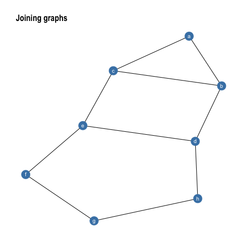
The standard dplyr verbs protects the to and from columns in the edge data
in order to avoid accidental modification of the graph topology. If changing of
the terminal nodes are necessary the reroute() verb will come in handy:
gr1 <- create_star(6, directed = TRUE)
layout <- create_layout(gr1, layout = 'fr')
gr1 <- gr1 %>%
    mutate(x = layout$x, y = layout$y, graph = 'original')
gr2 <- gr1 %>%
    mutate(graph = 'reverse') %>%
    activate(edges) %>%
    reroute(from = to, to = from)
gr3 <- gr1 %>%
    mutate(graph = 'using subset') %>%
    activate(edges) %>%
    reroute(from = to + 1, subset = to < 4)
ggraph(bind_graphs(gr1, gr2, gr3), layout = 'nicely') +
    geom_edge_link(arrow = arrow()) +
    facet_nodes(~graph) +
    theme_graph(foreground = 'steelblue')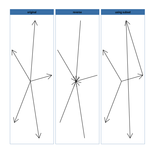
As can be seen, reroute works pretty much as a to and from specific
mutate(), with the added benefit of incorporating a subset operator if only a
few edges should be changed.
Making the most of graphs
While being able to use the dplyr verbs on relational data is nice and all,
one of the reasons we are dealing with graph data in the first place is because
we need some graph-based algorithms for solving our problem at hand. If we need
to break out of the tidy workflow every time this was needed we wouldn’t have
gained much. Because of this tidygraph has wrapped more or less all of
igraphs algorithms in different ways, ensuring a consistent syntax as well as
output that fits into the tidy workflow. In the following we’re going to take a
look at these.
Central to all of these functions is that they know about which graph is being
computed on (in the same way that n() knows about which tibble is currently in
scope). Furthermore they always return results matching the node or edge
position so they can be used directly in mutate() calls.
Node and edge types
On the top of our list of things we might be interested to know about is whether
nodes or edges are of specific types such as leaf, sink, loop,
etc. All of these functions return a logical vector indicating if the node or
edge belong to the specified group. To easily find functions that queries types,
all functions are prefixed with node_is_*/edge_is_*.
create_tree(20, 3) %>%
    mutate(leaf = node_is_leaf(), root = node_is_root()) %>%
    ggraph(layout = 'tree') +
    geom_edge_diagonal() +
    geom_node_point(aes(filter = leaf), colour = 'forestgreen', size = 10) +
    geom_node_point(aes(filter = root), colour = 'firebrick', size = 10) +
    theme_graph()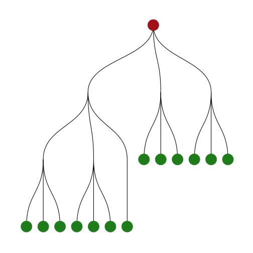
Another example could be to remove loop edges using filter(!edge_is_loop()).
Centrality
One of the simplest concepts when computing graph based values is that of
centrality, i.e. how central is a node or edge in the graph. As this
definition is inherently vague, a lot of different centrality scores exists that
all treat the concept of central a bit different. One of the famous ones is
the pagerank algorithm that was powering Google Search in the beginning.
tidygraph currently has 11 different centrality measures and all of these are
prefixed with centrality_* for easy discoverability. All of them returns a
numeric vector matching the nodes (or edges in the case of
centrality_edge_betweenness()).
play_smallworld(1, 100, 3, 0.05) %>%
    mutate(centrality = centrality_authority()) %>%
    ggraph(layout = 'kk') +
    geom_edge_link() +
    geom_node_point(aes(size = centrality, colour = centrality)) +
    scale_color_continuous(guide = 'legend') +
    theme_graph()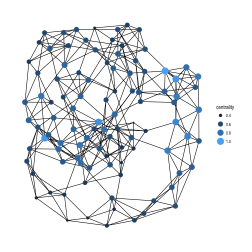
It is quite difficult to a priori decide which centrality measure makes most sense for a problem at hand so having easy access to a large range of them in a common syntax is a boon.
Clustering
Another common operation is to group nodes based on the graph topology,
sometimes referred to as community detection based on its commonality in social
network analysis. All clustering algorithms from igraph is available in
tidygraph using the group_* prefix. All of these functions return an integer
vector with nodes (or edges) sharing the same integer being grouped together.
play_islands(5, 10, 0.8, 3) %>%
    mutate(community = as.factor(group_infomap())) %>%
    ggraph(layout = 'kk') +
    geom_edge_link(aes(alpha = ..index..), show.legend = FALSE) +
    geom_node_point(aes(colour = community), size = 7) +
    theme_graph()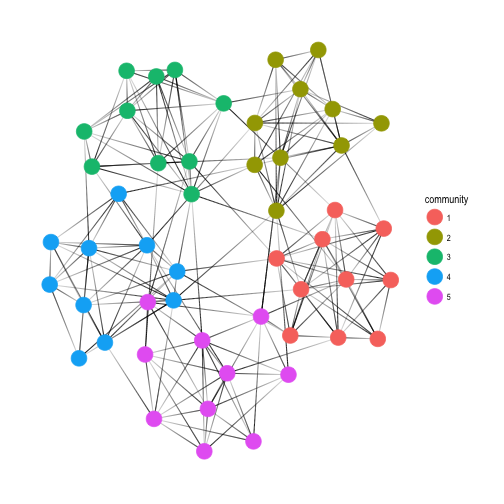
Node pairs
Some statistics are a measure between two nodes, such as distance or similarity
between nodes. In a tidy context one of the ends must always be the node defined
by the row, while the other can be any other node. All of the node pair
functions are prefixed with node_* and ends with _from/_to if the measure
is not symmetric and _with if it is; e.g. there’s both a node_max_flow_to()
and node_max_flow_from() function while only a single node_cocitation_with()
function. The other part of the node pair can be specified as an integer vector
that will get recycled if needed, or a logical vector which will get recycled
and converted to indexes with which(). This means that output from node type
functions can be used directly in the calls, e.g.
play_geometry(50, 0.25) %>%
    mutate(dist_to_center = node_distance_to(node_is_center())) %>%
    ggraph(layout = 'kk') +
    geom_edge_link() +
    geom_node_point(aes(size = dist_to_center), colour = 'steelblue') +
    scale_size_continuous(range = c(6, 1)) +
    theme_graph()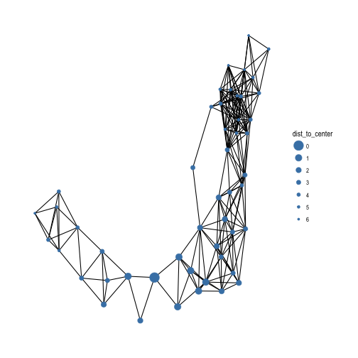
Searches
An integral type of operation on graphs is to perform a search, that is, start
from one node and then traverse the edges until all nodes has been visited. The
most common approaches are either breath first search where all neighbors of
a node is visited before moving on to the next node, or depth first serch
where you move along to the next node immediately and only backtracks and visit
other neighbors when you’ve hit a dead end. Different statistics from these
searches are available in tidygraph through the bfs_*() and dfs_*() family
of functions e.g. the distance to the start node along the search can be
obtained with bfs_dist()/dfs_dist(). The root node can be specified in the
same way as with node pairs. Sorting based on a search from the node with
highest centrality can thus be done with:
play_geometry(50, 0.25) %>%
    mutate(order = bfs_rank(which.max(centrality_alpha())))
#> # A tbl_graph: 50 nodes and 227 edges
#> #
#> # An undirected simple graph with 1 component
#> #
#> # Node Data: 50 x 3 (active)
#> x y order
#> <dbl> <dbl> <int>
#> 1 0.01637861 0.11280499 49
#> 2 0.01721270 0.19181732 50
#> 3 0.02015524 0.74802650 46
#> 4 0.04361792 0.09377818 48
#> 5 0.04622344 0.95686281 47
#> 6 0.07677761 0.46011354 41
#> # ... with 44 more rows
#> #
#> # Edge Data: 227 x 2
#> from to
#> <int> <int>
#> 1 1 2
#> 2 1 4
#> 3 2 4
#> # ... with 224 more rowsLocal measures
Often we find ourselves interested in the local neighborhood of a node for
various reasons. We might want to know the average degree around a node or the
number of triangles each node participate in. The local_*() family of
functions provide access to a range of node measures that are dependent on the
local neighborhood of each node.
# Weight the node degree by the average degree of its neighboors
play_smallworld(1, 100, 3, 0.05) %>%
    mutate(weighted_degree = centrality_degree() / local_ave_degree())
#> # A tbl_graph: 100 nodes and 300 edges
#> #
#> # An undirected simple graph with 1 component
#> #
#> # Node Data: 100 x 1 (active)
#> weighted_degree
#> <dbl>
#> 1 1.0000000
#> 2 1.0000000
#> 3 0.6666667
#> 4 1.2549020
#> 5 1.0000000
#> 6 1.0000000
#> # ... with 94 more rows
#> #
#> # Edge Data: 300 x 2
#> from to
#> <int> <int>
#> 1 1 2
#> 2 2 3
#> 3 4 97
#> # ... with 297 more rowsAll the rest
While an ontology of graph operations has been attempted in the different
functions above, there are some that falls outside. These have been lumped
together under the node_*() and edge_*() umbrellas and include things such
as topological ordering and Burt’s constraint among others. All of these
functions ensures a mutate-compatible output.
Graph measures
Along with computations on the individual nodes and edges it is sometimes
necessary to get summary statistics on the graph itself. These can be simple
measures such as the number of nodes and edges as well as more involved measures
such as assortativity (the propensity of similar nodes to be connected). All of
these measures can be calculated through the graph_*() function family and
they will all return a scalar.
# Normalise the node pair adhesion with the minimal adhesion of the graph
play_islands(5, 10, 0.7, 3) %>%
    mutate(norm_adhesion = node_adhesion_to(c(50, 1:49)) / graph_adhesion())
#> # A tbl_graph: 50 nodes and 183 edges
#> #
#> # An undirected simple graph with 1 component
#> #
#> # Node Data: 50 x 1 (active)
#> norm_adhesion
#> <dbl>
#> 1 2.00
#> 2 1.75
#> 3 1.25
#> 4 1.25
#> 5 1.75
#> 6 1.75
#> # ... with 44 more rows
#> #
#> # Edge Data: 183 x 2
#> from to
#> <int> <int>
#> 1 1 2
#> 2 2 3
#> 3 1 4
#> # ... with 180 more rowsMapping over nodes
Just to spice it all up a bit tidygraph pulls purrr into the mix and
provides some additional graph-centric takes on the familiar map*(). More
specifically tidygraph provides functionality to apply a function over nodes
as a breath or depth first search is carried out, while getting access to the
result of the computations coming before, as well as mapping over the local
neighborhood of each node. All of these function returns a list in their
bare bone form, but as with purrr versions exists that ensures the output is of
a certain type (e.g. map_bfs_dbl()).
Mapping over searches
The search maps comes in two flavors. Either the nodes are mapped in the order of the search, or they are mapped in the reverse order. In the first version, each call will have access to the statistics and map results of all the nodes that lies between itself and the root. In the second version each call will have access to the results and statistics of all its offspring. Furthermore the mapping function is passed the graph itself as well as all the search statistics of the node currently being mapped over. An example would be to propagate the species value in our iris clustering upwards as long as theirs agreement between the children. For this to work, we will need the reverse version of a breath first search to make sure that all children have been evaluated prior to mapping over a node:
iris_tree <- iris_tree %>%
    activate(nodes) %>%
    mutate(Species = map_bfs_back_chr(node_is_root(), .f = function(node, path, ...) {
        nodes <- .N()
        if (nodes$leaf[node]) return(nodes$Species[node])
        if (anyNA(unlist(path$result))) return(NA_character_)
        path$result[[1]]
    }))
ggraph(iris_tree, layout = 'dendrogram') +
    geom_edge_diagonal2(aes(colour = node.Species)) +
    theme_graph()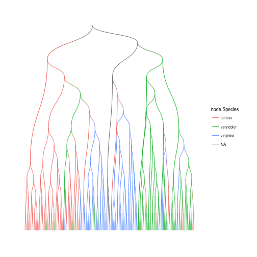
Mapping over neighborhoods
The neighborhood map is exposed through map_local() as well as its type safe
versions. The mapping function has a much simpler format as it simply gets
passed a subgraph representing the local neighborhood as well as the index of
the node in the original graph being mapped over. E.g. to get the number of
edges in the local neighborhood around each node, one would simply do:
play_smallworld(1, 100, 3, 0.05) %>%
    mutate(neighborhood_edges = map_local_dbl(.f = function(neighborhood, ...) {
        igraph::gsize(neighborhood)
    }))
#> # A tbl_graph: 100 nodes and 300 edges
#> #
#> # An undirected simple graph with 1 component
#> #
#> # Node Data: 100 x 1 (active)
#> neighborhood_edges
#> <dbl>
#> 1 14
#> 2 14
#> 3 14
#> 4 13
#> 5 15
#> 6 15
#> # ... with 94 more rows
#> #
#> # Edge Data: 300 x 2
#> from to
#> <int> <int>
#> 1 1 2
#> 2 2 3
#> 3 3 4
#> # ... with 297 more rowsOne last thing…
While the functions discussed above makes it easy to make slight changes to your
network topology it is less straightforward to make radical changes. Even more
so if the radical changes are only needed temporarily for the sake of a few
computations. This is where the new morph() verb comes in handy (along with
the accompanying unmorph() and crystallise() verbs). In essence, morph()
lets you set up a temporary alternative version of your graph, make computations
on it using the standard dplyr verbs, and then merge the changes back in
using unmorph(). The types of alternative representations are varied and can
be extended by the user. Nodes can be converted to edges and the other way
around, both nodes and edges can be combined, and the alternate representation
does not need to cover the full original graph. Instead of trying to describe it
in words, let’s see how it plays out in use:
islands <- play_islands(5, 10, 0.8, 3) %>%
    mutate(group = group_infomap())

# Get the distance to the central node in each group
islands <- islands %>%
    morph(to_split, group) %>%
    mutate(dist_to_center = node_distance_to(node_is_center())) %>%
    unmorph()
islands
#> # A tbl_graph: 50 nodes and 208 edges
#> #
#> # An undirected simple graph with 1 component
#> #
#> # Node Data: 50 x 2 (active)
#> group dist_to_center
#> <int> <dbl>
#> 1 3 1
#> 2 3 1
#> 3 3 1
#> 4 3 1
#> 5 3 0
#> 6 3 1
#> # ... with 44 more rows
#> #
#> # Edge Data: 208 x 2
#> from to
#> <int> <int>
#> 1 1 2
#> 2 1 3
#> 3 2 3
#> # ... with 205 more rows# Get the number of edges exiting each group
islands <- islands %>%
morph(to_contracted, group, simplify = FALSE) %>%
activate(edges) %>%
filter(!edge_is_loop()) %>%
activate(nodes) %>%
mutate(exiting_group = centrality_degree(mode = 'out')) %>%
unmorph()
islands#> # A tbl_graph: 50 nodes and 208 edges
#> #
#> # An undirected simple graph with 1 component
#> #
#> # Node Data: 50 x 3 (active)
#> group dist_to_center exiting_group
#> <int> <dbl> <dbl>
#> 1 3 1 12
#> 2 3 1 12
#> 3 3 1 12
#> 4 3 1 12
#> 5 3 0 12
#> 6 3 1 12
#> # ... with 44 more rows
#> #
#> # Edge Data: 208 x 2
#> from to
#> <int> <int>
#> 1 1 2
#> 2 1 3
#> 3 2 3
#> # ... with 205 more rows# Calculate an edge centrality score by converting to the linegraph
islands <- islands %>%
morph(to_linegraph) %>%
activate(nodes) %>%
mutate(edge_centrality = centrality_pagerank()) %>%
unmorph()
islands#> # A tbl_graph: 50 nodes and 208 edges
#> #
#> # An undirected simple graph with 1 component
#> #
#> # Node Data: 50 x 3 (active)
#> group dist_to_center exiting_group
#> <int> <dbl> <dbl>
#> 1 3 1 12
#> 2 3 1 12
#> 3 3 1 12
#> 4 3 1 12
#> 5 3 0 12
#> 6 3 1 12
#> # ... with 44 more rows
#> #
#> # Edge Data: 208 x 3
#> from to edge_centrality
#> <int> <int> <dbl>
#> 1 1 2 0.004220249
#> 2 1 3 0.004490694
#> 3 2 3 0.003728624
#> # ... with 205 more rowsAs can be seen, the morph syntax both handles multiple graphs, collapsed nodes
and changing edges to nodes, without any change in the mental model of the
operations. All morphing functions are prefixed with to_* for easy discovery
and includes minimum spanning trees, complement graph, dominator tree etc. In
the case where you are interested to continue working with the morphed
representation as a proper tbl_graph you can use the cystallise() verbs that
removes any link to the original graph and returns a tibble with a row per graph
in the morphed representation (as a morph can result in multiple graphs):
islands %>%
    morph(to_split, group) %>%
    crystallise()
#> # A tibble: 5 x 2
#> name graph
#> <chr> <list>
#> 1 group: 1 <S3: tbl_graph>
#> 2 group: 2 <S3: tbl_graph>
#> 3 group: 3 <S3: tbl_graph>
#> 4 group: 4 <S3: tbl_graph>
#> 5 group: 5 <S3: tbl_graph>Wrapping it all up
I hope I have given you a small glimpse of what tidygraph is all about. If
working with network data in the past has felt intimidating and strange
tidygraph might feel more at home, but even if you’re a seasoned pro within
network analysis the package should provide a powerful but streamlined interface
to many operations.
Roadmap
The next goal of my quest to revamp relational data analysis in R will be to
“rebuild” ggraph around tidygraph. This is not to say that the two are
incompatible at the moment — there’s full support through ggraphs support for
igraph — rather I want to only support tbl_graph in the future as all
relevant data structures can be converted to this common format through
as_tbl_graph().
For tidygraph itself, I have some more ideas I want to explore. Currently
missing from the whole package is any notion of modelling and it will be
interesting to see how this can fit in. Further, I have this wild idea about
providing a tidygraph link to graph databases such as Neo4J in the same way
as dbplyr provides an interface to SQL databases. Lastly, the current focus
has been on supporting the algorithms provided by igraph. While an extensive
package, igraph does not implement everything and there might be stuff lacking
that should be added down the line.
Take care…