Introduction to ggraph: Layouts

I will soon submit ggraph to CRAN - I swear! But in the meantime I’ve decided to build up anticipation for the great event by publishing a range of blog posts describing the central parts of ggraph: Layouts, Nodes, Edges, and Connections. All of these posts will be included with ggraph as vignettes — potentially in slightly modified form. To kick off everything we’ll start with the first thing you’ll have to think about when plotting a graph structure…

Layouts

In very short terms, a layout is the vertical and horizontal placement of nodes when plotting a particular graph structure. Conversely, a layout algorithm is an algorithm that takes in a graph structure (and potentially some additional parameters) and return the vertical and horizontal position of the nodes. Often, when people think of network visualizations, they think of node-edge diagrams where strongly connected nodes are attempted to be plotted in close proximity. Layouts can be a lot of other things too though — e.g. hive plots and treemaps. One of the driving factors behind ggraph has been to develop an API where any type of visual representation of graph structures is supported. In order to achieve this we first need a flexible way of defining the layout…

ggraph() and create_layout()

As the layout is a global specification of the spatial position of the nodes it spans all layers in the plot and should thus be defined outside of calls to geoms or stats. In ggraph it is often done as part of the plot initialization using ggraph() — a function equivalent in intent to ggplot(). As a minimum ggraph() must be passed a graph object supported by ggraph:

library(ggraph)
library(igraph)
graph <- graph_from_data_frame(highschool)

# Not specifying the layout - defaults to "auto"
ggraph(graph) + 
    geom_edge_link(aes(colour = factor(year))) + 
    geom_node_point()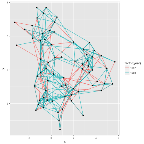

Not specifying a layout will make ggraph pick one for you. This is only intended to get quickly up and running. The choice of layout should be deliberate on the part of the user as it will have a great effect on what the end result will communicate. From now on all calls to ggraph() will contain a specification of the layout:

ggraph(graph, layout = 'kk') + 
    geom_edge_link(aes(colour = factor(year))) + 
    geom_node_point()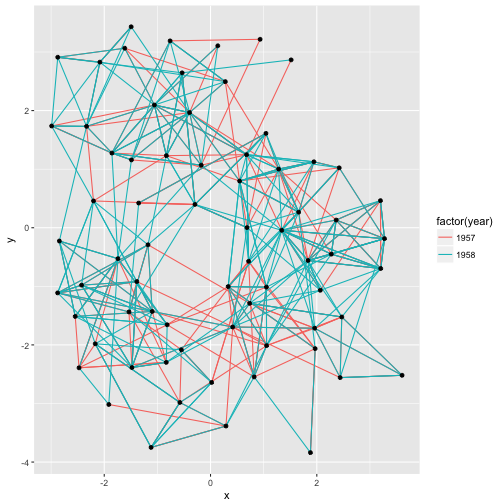

If the layout algorithm accepts additional parameters (most do), they can be supplied in the call to ggraph() as well:

ggraph(graph, layout = 'kk', maxiter = 100) + 
    geom_edge_link(aes(colour = factor(year))) + 
    geom_node_point()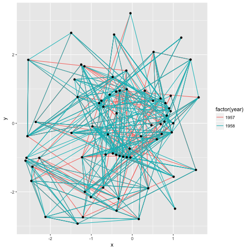

In addition to specifying the layout during plot creation it can also happen separately using create_layout(). This function takes the same arguments as ggraph() but returns a layout_ggraph object that can later be used in place of a graph structure in ggraph call:

layout <- create_layout(graph, layout = 'drl')
ggraph(layout) + 
    geom_edge_link(aes(colour = factor(year))) + 
    geom_node_point()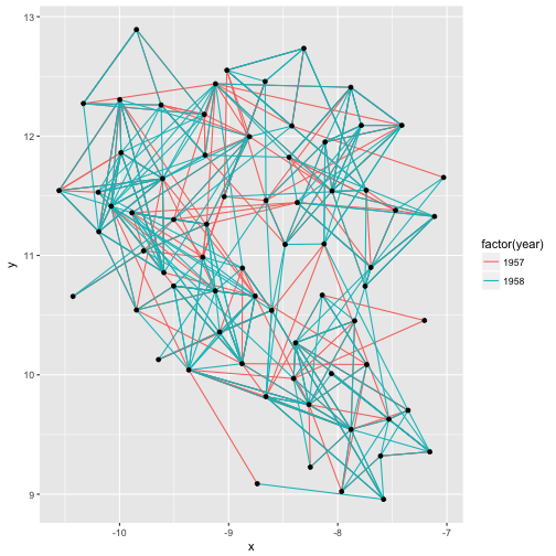

Examining the return of create_layout() we see that it is really just a data.frame of node positions and (possible) attributes. Furthermore the original graph object along with other relevant information is passed along as attributes:

head(layout)

#>           x         y name circular ggraph.index
#> 1 -7.734004 10.085789    1    FALSE            1
#> 2 -8.251559  9.226503    2    FALSE            2
#> 3 -7.205127 10.455535    3    FALSE            3
#> 4 -7.113050 11.326465    4    FALSE            4
#> 5 -7.748919 10.742258    5    FALSE            5
#> 6 -7.355531  9.702643    6    FALSE            6

attributes(layout)

#> $names
#> [1] "x"            "y"            "name"         "circular"    
#> [5] "ggraph.index"
#> 
#> $row.names
#>  [1]  1  2  3  4  5  6  7  8  9 10 11 12 13 14 15 16 17 18 19 20 21 22 23
#> [24] 24 25 26 27 28 29 30 31 32 33 34 35 36 37 38 39 40 41 42 43 44 45 46
#> [47] 47 48 49 50 51 52 53 54 55 56 57 58 59 60 61 62 63 64 65 66 67 68 69
#> [70] 70
#> 
#> $class
#> [1] "layout_igraph" "layout_ggraph" "data.frame"   
#> 
#> $graph
#> IGRAPH DN-- 70 506 -- 
#> + attr: name (v/c), year (e/n)
#> + edges (vertex names):
#>  [1] 1 ->14 1 ->15 1 ->21 1 ->54 1 ->55 2 ->21 2 ->22 3 ->9  3 ->15 4 ->5 
#> [11] 4 ->18 4 ->19 4 ->43 5 ->19 5 ->43 6 ->13 6 ->20 6 ->22 7 ->17 8 ->14
#> [21] 8 ->17 9 ->12 9 ->20 9 ->21 9 ->22 9 ->51 11->19 11->50 11->52 11->53
#> [31] 12->20 12->21 12->22 13->17 13->20 13->21 13->22 14->21 14->22 15->20
#> [41] 16->18 16->41 16->43 17->7  17->8  18->11 18->16 18->19 19->4  19->11
#> [51] 19->16 19->18 19->27 20->6  20->12 20->21 20->22 20->38 21->22 21->51
#> [61] 21->54 21->55 22->20 22->21 22->38 22->51 23->40 23->43 23->50 23->52
#> [71] 23->53 23->60 23->62 23->65 23->68 24->51 26->32 26->35 26->36 26->40
#> + ... omitted several edges
#> 
#> $circular
#> [1] FALSE

As it is just a data.frame it means that any standard ggplot2 call will work by addressing the nodes. Still, use of the geom_node_*() family provided by ggraph is encouraged as it makes it explicit which part of the data structure is being worked with.

Adding support for new data sources

Out of the box ggraph supports dendrogram and igraph objects natively as well as hclust and network through conversion to one of the above. If there is wish for support for additional classes this can be achieved by adding a set of specific methods to the class. The ggraph source code should be your guide in this but I will briefly describe the methods below:

create_layout.myclass()

This method is responsible for taking a graph structure and returning a layout_ggraph object. The object is just a data.frame with the correct class and attributes added. The class should be c('layout_myclass', 'layout_ggraph', 'data.frame') and it should at least have a graph attribute holding the original graph object as well as a circular attribute with a logical giving whether the layout has been transformed to a circular representation or not. If the graph structure contains any additional information about the nodes this should be added to the data.frame as columns so these are accessible during plotting.

getEdges.layout_myclass()

This method takes the return value of create_layout.myclass() and returns the edges of the graph structure. The return value should be in the form of an edge list with a to and from column giving the indexes of the terminal nodes of the edge. Furthermore, it must contain a circular column, again indicating whether the layout should be considered circular. If there are any additional data attached to the edges in the graph structure these should be added as columns to the data.frame.

getConnection.layout_myclass()

This method is intended to return the shortest path between two nodes as a list of node indexes. This method can be ignored but will result in lack of support for geom_conn_* layers.

layout_myclass_*()

Any type of layout algorithm that needs to be available to this class should be defined as a separate layout_myclass_layoutname() function. This function will be called when 'layoutname' is used in the layout argument in ggraph() or create_layout(). At a minimum each new class should have a layout_myclass_auto() defined.

Layouts abound

There’s a lot of different layouts in ggraph — first and foremost because igraph implements a lot of layouts for drawing node-edge diagrams and all of these are available in ggraph. Additionally, ggraph provides a lot of new layout types and algorithms for your drawing pleasure.

A note on circularity

Some layouts can be shown effectively both in a standard Cartesian projection as well as in a polar projection. The standard approach in ggplot2 has been to change the coordinate system with the addition of e.g. coord_polar(). This approach — while consistent with the grammar — is not optimal for ggraph as it does not allow layers to decide how to respond to circularity. The prime example of this is trying to draw straight lines in a plot using coord_polar(). Instead circularity is part of the layout specification and gets communicated to the layers with the circular column in the data, allowing each layer to respond appropriately. Sometimes standard and circular representations of the same layout get used so often that they get different names. In ggraph they’ll have the same name and only differ in whether or not circular is set to TRUE:

# An arc diagram
ggraph(graph, layout = 'linear') + 
    geom_edge_arc(aes(colour = factor(year)))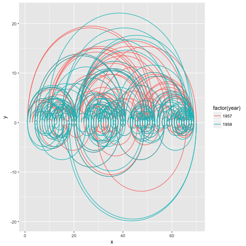

# A coord diagram
ggraph(graph, layout = 'linear', circular = TRUE) + 
    geom_edge_arc(aes(colour = factor(year)))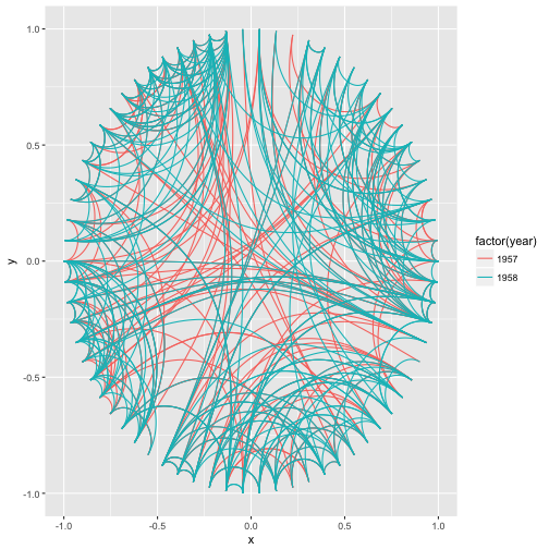

graph <- graph_from_data_frame(flare$edges, vertices = flare$vertices)
# An icicle plot
ggraph(graph, 'partition') + 
    geom_node_tile(aes(fill = depth), size = 0.25)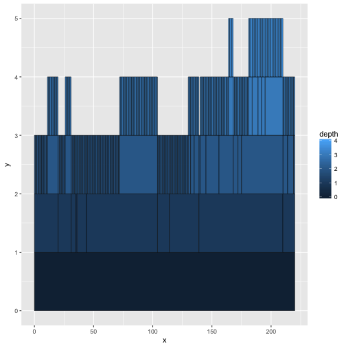

# A sunburst plot
ggraph(graph, 'partition', circular = TRUE) + 
    geom_node_arc_bar(aes(fill = depth), size = 0.25)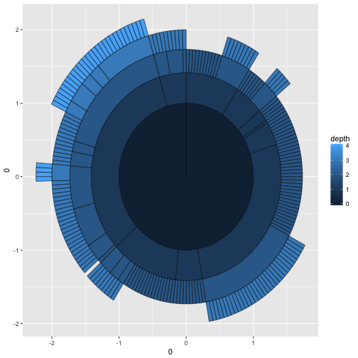

Not every layout has a meaningful circular representation in which cases the circular argument will be ignored.

Node-edge diagram layouts

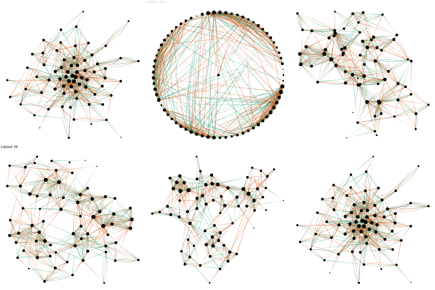
igraph provides a total of 13 different layout algorithms for classic node-edge diagrams (colloquially referred to as hairballs). Some of these are incredibly simple such as randomly, grid, circle, and star, while others tries to optimize the position of nodes based on different characteristics of the graph. There is no such thing as “the best layout algorithm” as algorithms have been optimized for different scenarios. Experiment with the choices at hand and remember to take the end result with a grain of salt, as it is just one of a range of possible “optimal node position” results. Below is an animation showing the different results of running all applicable igraph layouts on the highschool graph.

library(tweenr)
igraph_layouts <- c('star', 'circle', 'gem', 'dh', 'graphopt', 'grid', 'mds', 
                    'randomly', 'fr', 'kk', 'drl', 'lgl')
igraph_layouts <- sample(igraph_layouts)
graph <- graph_from_data_frame(highschool)
V(graph)$degree <- degree(graph)
layouts <- lapply(igraph_layouts, create_layout, graph = graph)
layouts_tween <- tween_states(c(layouts, layouts[1]), tweenlength = 1, 
                              statelength = 1, ease = 'cubic-in-out', 
                              nframes = length(igraph_layouts) * 16 + 8)
title_transp <- tween_t(c(0, 1, 0, 0, 0), 16, 'cubic-in-out')[[1]]
for (i in seq_len(length(igraph_layouts) * 16)) {
    tmp_layout <- layouts_tween[layouts_tween$.frame == i, ]
    layout <- igraph_layouts[ceiling(i / 16)]
    title_alpha <- title_transp[i %% 16]
    p <- ggraph(graph, 'manual', node.position = tmp_layout) + 
        geom_edge_fan(aes(alpha = ..index.., colour = factor(year)), n = 15) +
        geom_node_point(aes(size = degree)) + 
        scale_edge_color_brewer(palette = 'Dark2') + 
        ggtitle(paste0('Layout: ', layout)) + 
        theme_void() + 
        theme(legend.position = 'none', 
              plot.title = element_text(colour = alpha('black', title_alpha)))
    plot(p)
}

Hive plots

A hive plot, while still technically a node-edge diagram, is a bit different from the rest as it uses information pertaining to the nodes, rather than the connection information in the graph. This means that hive plots, to a certain extend is more interpretable as well as less vulnerable to small changes in the graph structure. They are less common though, so use will often require some additional explanation.

V(graph)$friends <- degree(graph, mode = 'in')
V(graph)$friends <- ifelse(V(graph)$friends < 5, 'few', 
                           ifelse(V(graph)$friends >= 15, 'many', 'medium'))
ggraph(graph, 'hive', axis = 'friends', sort.by = 'degree') + 
    geom_edge_hive(aes(colour = factor(year), alpha = ..index..)) + 
    geom_axis_hive(aes(colour = friends), size = 3, label = FALSE) + 
    coord_fixed()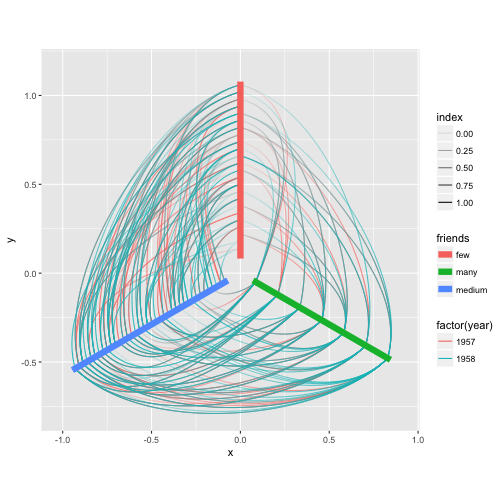

Hierarchical layouts

Trees and hierarchies are an important subset of graph structures, and ggraph provides a range of layouts optimized for their visual representation. Some of these uses enclosure and position rather than edges to communicate relations (e.g. treemaps and circle packing). Still, these layouts can just as well be used for drawing edges if you wish to:

graph <- graph_from_data_frame(flare$edges, vertices = flare$vertices)
set.seed(1)
ggraph(graph, 'circlepack', weight = 'size') + 
    geom_node_circle(aes(fill = depth), size = 0.25, n = 50) + 
    coord_fixed()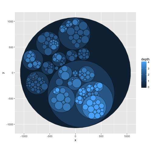

set.seed(1)
ggraph(graph, 'circlepack', weight = 'size') + 
    geom_edge_link() + 
    geom_node_point(aes(colour = depth)) +
    coord_fixed()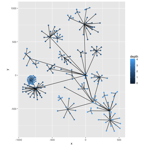

ggraph(graph, 'treemap', weight = 'size') + 
    geom_node_tile(aes(fill = depth), size = 0.25)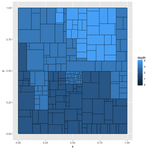

ggraph(graph, 'treemap', weight = 'size') + 
    geom_edge_link() + 
    geom_node_point(aes(colour = depth))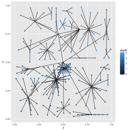

The most recognized tree plot is probably dendrograms though. Both igraph and dendrogram object can be plotted as dendrograms, though only dendrogram objects comes with a build in height information for placing the branch points. For igraph objects this is inferred by the longest ancestral length:

ggraph(graph, 'dendrogram') + 
    geom_edge_diagonal()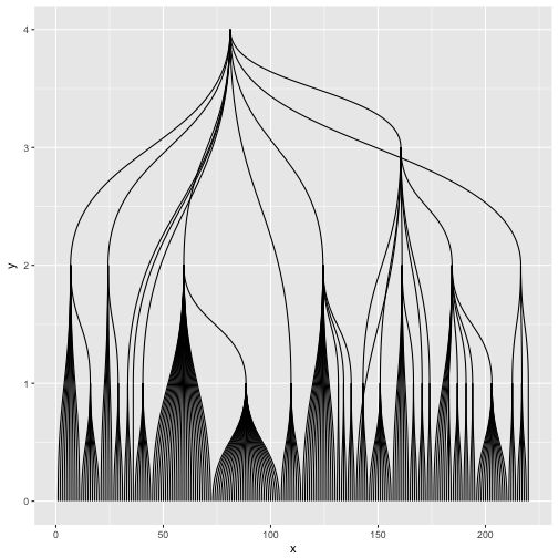

dendrogram <- as.dendrogram(hclust(dist(iris[, 1:4])))
ggraph(dendrogram, 'dendrogram') + 
    geom_edge_elbow()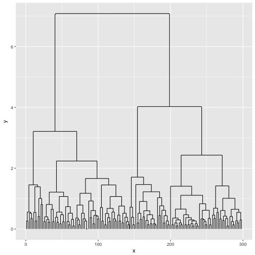

Dendrograms are one of the layouts that are amenable for circular transformations, which can be effective in giving more space at the leafs of the tree at the expense of the space given to the root:

ggraph(dendrogram, 'dendrogram', circular = TRUE) + 
    geom_edge_elbow() + 
    coord_fixed()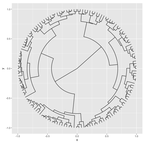

More to come

This concludes the first of the introduction posts about ggraph. I hope I have been effective in describing the use of layouts and illustrating how they can have a very profound effect on the resulting plot. Stay tuned for more…

Update

• ggraph Introduction: Nodes has been published